Simple example for computing spectra and lightcurve

All examples are available in examples folder as jupyter notebooks. In order to work with the package we recommend to import the following blocks and packages:

from magpies import *
from atmos import *
import numpy as np
from math import *

First we specify mass and radius of neutron star. These parameters will enter nearly every function because they define the compactness parameter and affect how light is emitted and propagated in close vicinity of the neutron star. Following the usual practise of the field mass is specified in units of solar mass and radius is in km. It is also useful to choose polar magnetic field Bp [G] and temperature in deep layers of neutron stars Tb [K].

# Radius and mass of neutron star
Rns = 12  ## km
Mns = 1.4 ## M_solar
Tb = pow(10, 7.1730)  ## K
Bp = 1e11 ## G

Now we compute free fall acceleration and initialise the iron atmosphere following fit from Potekhin et al. (2003) article for dipolar magnetic field.

g14c = g14 (Rns, Mns) ## computing the free fall acceleration
atm_iron_2003 = NS_atmosphere ('Potekhin_2003_iron', g14c, Tb, Bp)
atm_iron_2003.describe ()

The function g14() is a part of Magpies library while NS_atmosphere() is a class from the Atmos library. The method describe() simply provide more details about the fit and relevant literature reference.

Further we create a surface temperature distribution map, see more details in Initialising the surface thermal map

Tm = Tmap (usage='NS_atm', ns_atm=atm_iron_2003)

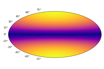
The class Tmap creates a member which stores coordinates of the surface mesh and values of the temperature in these points. In this particular case, the class uses NS_atmosphere to compute values of temperature. We can plot the surface thermal map in Aitoff projection using method atmos.Tmap.plot_Ts:

Tm.plot_Ts()

We normally transpose the temperature array using numpy method .T. The result is shown below.

Now when the surface thermal map is prepared we can try different functions from the Magpies package. For example the package has basic functionality which allows fast calculations of total thermal luminosity and effective temperature

L    = compute_L(Tm, Rns)
Teff = compute_Teff(Tm, Rns)
print ('L = ', L, ' Teff = ', Teff)

This function gives \(L = 6.7\times 10^{30}\) erg/s and \(T_\mathrm{eff} = 2.8\times 10^5\) K. Advanced methods available in Magpies package allows to compute the spectra:

eph = np.logspace (-1.2, 1.62, 142) ## keV

spect, visib = spectra_pole (Tm, Rns, Mns, eph)

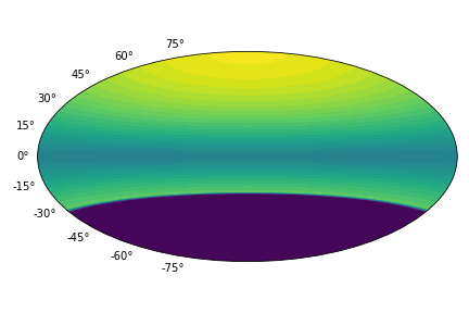
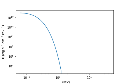
Here eph is list of energies where the spectra is computed, spect is the effective spectral flux and visib shows the temperature distribution over the visible hemisphere. We can plot the resulting spectra as the following:

plt.plot (eph, spect)
plt.xlabel('E (keV)')
plt.ylabel(r'H (erg s$^{-1}$ cm$^{-2}$ keV$^{-1}$)')
plt.ylim([1, 1e20])
plt.xscale('log')
plt.yscale('log')

Which gives us the following plot.

The visible map looks like the following:

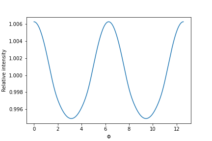
It is possible to create a lightcurve.

phases = np.linspace (0, 4*pi, 400)
intens = lightcurve (Tm, Rns, Mns, phases, 0, pi/4)

intens_rel = np.asarray(intens) / np.mean(intens)

plt.plot (phases, intens_rel)
plt.xlabel(r'$\Phi$')
plt.ylabel('Relative intensity')
plt.savefig('lightcurve.png')